Computer Vision

My notes for CS4243

L7,L8,L9 Keypoints notes

Combining 2 images

Find keypoints / interest points / corners / Harris Corners

• Preferably Invariant to transformations (if it is affected = equivariant)
  • Geometric (warping img transformation):
  • Translation & Rotation: KP Location not invariant, Harris Corner resp. invariant
  • Scale: Corner response not invariant
    • To counter: slowly scale image from small to big and find scale for which response R is the largest
    • Instead of continuous scales, we can use the gaussian pyramid method
    • Instead of using Harris Corner response (expensive to run on all pixels), we can use LoG as a response on the image to find the scale (note: only to find the scale, LoG looks for edges not corners specifically)
      • https://automaticaddison.com/how-the-laplacian-of-gaussian-filter-works/
      • Find 1st derivative of image to find gradients
      • Sensitive to noise, so instead use 2nd derivative of image (edge at 0)
        • Both sensitive to noise, so apply gaussian filter first, then Laplacian (thus LoG)
        • Extra: Found in W4 L4 gradients.pdf
        • Approximate LoG using Difference of Gaussian (using Gaussian pyramid)
  • Photometric (filtering img transformation):
  • Intensity changes:
    • Difference is the same: response invariant
    • Otherwise response not invariant (is heavily dependent on gradient intensity due to thresholding, L7S38)
• Distinct from other descriptors (Harris Corners)
  • Look for corners (significant gradient in all directions)
  • Find pixel I(x,y) with highest intensity difference w.r.t. all surrounding pixels I(x+u,y+v) based on window [Slide 15]
    • In practice, weighted by distance from center pixel (L7S31)
  • Approximate I(x+u,y+v) from I(x,y) using Taylor Series expansion up to 1st order approximation (L7S16)
  • Thus obtaining the 2nd moment matrix H at S17 and S18
  • Then, diagonalize the matrix and get its eigenvalues. These eigenvalues represent the horizontal and vertical gradient. We want both to be strong (thus response R = min(lambda1, lambda2))
    • Harris Operator: Since det(H) = lambda1 lambda2 and trace(H) = lambda1 + lambda2, R is approximated by det(H) - ktrace^2(H), if > 0 we call it a corner
  • Non-maximum suppression Get local maximum (maybe by window S28), then pick the maxima of the local maxima within a radius (S30)
• Efficient (Don't want too many)
• Small (robust to clutter and occlusion)

Compute feature descriptors (vectors) to mathematically represent these keypoints and their surrounding region

• Vector of pixel intensities: sensitive to any change
• Vector of gradients: sensitive to deformations
• Color histogram: invariant to scale & rotation, but more false matches
  • Spatial histograms: compute different histograms on patch split into grid: some invariance to deformations
    • To make sure rotation invariant, normalize orientation by finding dominant orientation (overall gradient), then rotate patch to that direction
      • Multi-Scale Oriented Patches (MOPS): To reduce effect of deformations, subsample parts of the patch, normalize then wavelet transform.
      • GIST: Compute Gabor filter bank histogram from each square in patch split into a grid
      • SIFT: 4 Steps
        • Benefits
          • Invariant to scale and rotation
        1. Find best scale for keypoints: Multi-Scale Extrema (Blob) Detection
        • Gaussian Pyramid (each level is an "octave" with scale decreasing by 1/2 per level)
        • At each level, discretely vary the sigma to calculate the difference of gaussian (to approx. LoG) and find local maxima
        2. Refine keypoint location to sub-pixel accuracy
        • Compute Harris Corner response (Hessian) of DoG image and keep maxima if HC response above threshold
        3. Rotate keypoints based on their dominant orientation
        4. Create descriptor
           • Re-weight gradient magnitudes for each pixel based on gaussian centered on keypoint, discard pixels with low magnitude
           • Split patch into grid, then create gradient orientation histogram (8 bins, 45deg per bin) for each square
           • Make sure descriptors aligned to dominant orientation, then normalize vector, clamp values, etc

Perform keypoint / feature matching

• Simple: Minimum SSD between the feature vectors
• Better: ratio distance 1stDiff:2ndDiff (smaller the better)
  • dist(kp_in_imgA - bestKp_in_imgB) / dist(kp_in_imgA - 2ndBestKp_in_imgB)
• Test this feature in img_A with all other features in img_B using indexing structure
• Set a threshold, which affects
  • Precision: % of matches being true matches [TP / (TP + FP)]
    • Higher threshold = more lax = lower precision
  • Recall: % of all true matches found [TP / (TP + FN)]
    • Higher threshold = more lax = higher recall
  • Specificity: % of all false matches discarded [TN / (TN + FP)]
    • Higher threshold = more lax = lower specificity

Perform a transformation on img_B to merge it with img_A using the keypoint matches {p,p'}

• If {p,p'} is a correct match, then p = a H p'
  • p = [x, y, z]^T where z=1, .: [x, y, z]^T
  • a is an unknown scale factor
  • H is a 3x3 homography matrix (See L9 S10)
    • See what is a homography
      • Isometric transformations (just skip through)
        • How it is related to the matrix
        • Last row (0,0,1) to preserve z = 1
      • Similarity: same as isometric but with scale
      • Affine: skew
      • Projective / homography:
      • Perspective transformation: 1 level above
  • 4 pairs needed to calculate a concrete H matrix as it has 8 degrees of freedom
    • Solve using normalized DLT
  • Outliers (bad matches) will significantly affect the DLT, so do Random Sampling Consensus (RANSAC)
    • RANSAC: General algorithm to estimate best parameters to fit model to inliners (S20)
      • Randomly sample minimum points required to fit model
      • Solve for model parameters using samples
      • Count number of points (inliers) that are covered by the model (using a threshold) using the params found
      • Choose the params that cover the most points after iterating N times
      • Formula for N based on % of inliers and confidence % of iteration without outliers on S24

Refresher on Gaussian, Laplacian of Gaussian & Difference of Gaussian

• Gaussian: Standard distribution but on 3D space (imagine x-axis now on x and y axis)
• Laplacian of Gaussian = 2nd derivative of gaussian
  • See https://i.stack.imgur.com/u8I01.png
  • https://automaticaddison.com/how-the-laplacian-of-gaussian-filter-works/
• Difference of Gaussian: Difference of image blurred with gaussians of different sigma
  • Approximation for the LoG
  • See https://en.wikipedia.org/wiki/Difference_of_Gaussians

L10, L11, 12

Tracking

• Estimate 2D / 3D position of object in a video (vid1)
  • 2D / 3D position: "parameters"
  • object: "system" consisting of feature points

Possible Methods:

1. Optical flow (translation transformation only)
2. Template matching
   • Find a target image in the image
     • Using normalized cross-correlation
     • Using LK Alignment (Optical flow w/ Affine transformations)
     • Or using Mean-shift tracking

Basic Optical flow

• Follow pixel based on its translation movement
• Only reliable for small movements
• Easily messed up with occlusions or textureless regions

Normalized X-correlation

• Method 1: Normalized Cross-Correlation
  • Cross-correlating an image with a template of the image you want to find
    • Not normalized: Response is affected by base intensity of the image
    • Normalized: Local max of response is most likely location
  • Slow, combinatory, global (cross-correlate entire image)
• Method 2: Multi-scale template matching
  • Perform template matching on pyramid from small to large scale (scale for both img and template)
  • Do local search on areas of higher response
  • Faster, combinatory, locally optimal

Local Refinement

• Method 3: Local refinement based on initial guess
  • Fastest, Locally optimal
  • Definitions:
    • 2D image transformation: $W(x;p)$
      • x = position ($x = \begin{bmatrix}x \\ y\end{bmatrix}$)
      • p = transformation parameters = $\{p_1,...,p_N\}$
        • N is dependent on type of transformation (See below for transform x coordinate matrix)
        • Translation: W(x;p) = $\begin{bmatrix}x+p_1 \\ y+p_2\end{bmatrix}$ = $\begin{bmatrix}1 & 0 & p_1 \\ 0 & 1 & p_2\end{bmatrix}\begin{bmatrix}x \\ y \\ 1\end{bmatrix}$ = $\begin{bmatrix}1 & 0 & p_1 \\ 0 & 1 & p_2 \\ 0 & 0 & 1\end{bmatrix}\begin{bmatrix}x \\ y \\ 1\end{bmatrix}$
        • Affine: W(x;p) = $\begin{bmatrix}p_1x+p_2y+p_3 \\ p_4x+p_5y+p_6\end{bmatrix}$ = $\begin{bmatrix}p_1 & p_2 & p_3 \\ p_4 & p_5 & p_6 \\ 0 & 0 & 1\end{bmatrix}\begin{bmatrix}x \\ y \\ 1\end{bmatrix}$
      • Template Image $T(x)$, x is a pixel coordinate in frame T
      • Input Image $I(x)$, x is a pixel coordinate in frame I
      • Warp function W(x;p): Takes pixel x in coordinate frame of T and maps it to sub-pixel location W(x;p) in coordinate frame of I
        • i.e. Let's say you have a coordinate x w.r.t. coordinate frame T
        • T(x) gives you the pixel values (intensity) of its original position in the template
        • I(x) gives you the pixel values (intensity) of some position in the image that is unrelated to its real position in the template
        • I(W(x;p)) gives you the pixel values (intensity) of some position in the image that is most likely where:
          • If you were to map the template onto the image, that's where it would be if the template was mapped on the image
          • The warped coordinates is also referred to as $x' = W(x;p)$
            • $I(x') = I(W(x;p))$
          • https://www.ri.cmu.edu/pub_files/pub3/baker_simon_2004_1/baker_simon_2004_1.pdf
  • Then we can represent:
    • Warped Image: $I(W(x;p))$
    • Template Image: $T(x)$
  • Then assume lowest difference between the two and sum over all the results
    • $\min_p\sum_x [I(W(x;p)) - T(x)]^2$
    • We want to solve for p to find where the template will map to
    • Find warp parameters p s.t. SSD is minimized over all pixels in the template img
    • This is hard to optimize because I(W(x;p)) is not linear

LK Alignment

Lucss-Kanade (Additive) Alignment, which builds on the idea of local refinement; basically Optical Flow but using affine transformations instead of translation

• Paper

Theory

• Assuming we had a good initial guess on the params p
  • We can separate initial guess p and $\Delta p$ and minimize $\Delta p$
  • $\min_{\Delta p}\sum_x [I(W(x;p+\Delta p)) - T(x)]^2$
  • Since $\Delta p$ is small we can use Taylor Series approximation to linearise I(...)
    • Refresher: Multivariable Taylor Series Expansion (1st order approx)
      • $f(x,y)\approx f(a,b) + f_x(a,b)(x-a) + f_y(a,b)(y-b)$
      • $I(W(x;p+\Delta p))\approx I(W(x;p) + \frac{\delta I(W(x;p))}{\delta p}\Delta p$
      • Apply chain rule we get:
      • $I(W(x;p+\Delta p))\approx I(W(x;p) + \frac{\delta I(W(x;p))}{\delta W(x;p)}\Delta \frac{\delta W(x;p)}{\delta p}\Delta p$
      • Now recall that $x' = W(x;p)$, hence $\frac{\delta I(W(x;p))}{\delta W(x;p)}$ = gradient of I (i.e. $\nabla I$)
      • $I(W(x;p+\Delta p))\approx I(W(x;p) + \nabla I \frac{\delta W(x;p)}{\delta p}\Delta p$
        • $\frac{\delta W(x;p)}{\delta p}$ = Jacobian Matrix (Matrix of Partial Derivatives)
          • Refresher
            • Example: Affine: W(x;p) (See main formula above)
              • $\frac{\delta W(x;p)}{\delta p} = \begin{bmatrix}x & y & 1 & 0 & 0 & 0 \\ 0 & 0 & 0 & x & y & 1\end{bmatrix}$
          • Rate of change of the warp w.r.t. each warp param
  • And then we step out and get this:
  • $\approx \min_{\Delta p}\sum_x [I(W(x;p)+\nabla I \frac{\delta W(x;p)}{\delta p}\Delta p)) - T(x)]^2$
    • $\nabla I\equiv \frac{\delta I(W(x;p))}{\delta W(x;p)}$: Image gradient (1x2 vector); rate of change of pixel intensity at the warped coordinates w.r.t the warp
    • This is parallelizable (each coord. is independent)
  • Reshuffle to group the constants:
  • $\approx \min_{\Delta p}\sum_x [\nabla I \frac{\delta W(x;p)}{\delta p}\Delta p)) - [T(x) - I(W(x;p)]]^2$
  • $\approx \min_{\Delta p}\sum_x [Ax - b]]^2$
    • A is a constant vector ($\nabla I \frac{\delta W(x;p)}{\delta p}$)
    • x is a vector of variables ($\Delta p$)
    • b is a constant scalar ($[T(x) - I(W(x;p)]$)
  • Which we can use Least Square approximation to solve
    • Refresher: $\hat{x}=\argmin_x ||Ax-b||^2$ is solved by: $x=(A^TA)^{-1}A^Tb$
  • Using the simplified terms we introduced (A,x,b)
  • $\Delta p = H^{-1}\sum_x A^T b$
    • H is the Hessian Matrix (matrix of 2nd order derivative)
      • Approximated using Gauss-Newton
    • $H = \sum_x A^T A$

Methodology

Task	Eqn
Warp Image	$I(W(x;p))$
Compute Error Image (b)	$T(x) - I(W(x;p))$
Compute Gradient	$\nabla I(W(x;p)) \equiv \nabla I(x')$ (diff in intensity)
Evaluate Jacobian	$\frac{\delta (W(x;p))}{\delta p}$
Get vector "A"	$\nabla I \frac{\delta W(x;p)}{\delta p}$
Approximate Hessian	$H = \sum_x A^T A$, x: pixel coord
Compute $\Delta p$	$\Delta p = H^{-1}\sum_x A^T b$
Update params p	$p \rightarrow p + \Delta p$

This is the same as the Lucas-Kanade optical flow.

Using LK Alignment

1. Choose good features for tracking (corners) using harris corners
2. Loop over corners
3. Compute displacement to next frame using LK alignment
4. Store displacement of each corner, update corner position
5. (optional) Add more corners every M frames
6. Return long trajectories for each corner

Challenges for feature-based tracking

• Efficiency
• Accuracy
  • Changing appearances / disappearances

Feature Tracking & Optical Flow

• Optical Flow
  • Assuming brightness constancy, Calculate pixel movement
• Feature Tracking
  • Follows specific pixels as they move across multiple frames
  • Once we have features to track, we can use optical flow to track them

Mean-shift Tracking

Theory

• Given a target (template) and an image (filled with candidate pixels), find most likely position
  • Initial tracking often done manually
  • Assume that the matching box stays the same (scale) for this simplified version
  • Errors:
    • Catastrophic:
      • Occlusion
      • Exit frame
      • Multiple objects
    • Gradual:
      • Drifting
• Use Mean-shift clustering for tracking
  • Mean-shift clustering
  • 
    • imgsrc
  • (find mode / local density maxima in feature space)
    • For each datapoint
      • Define a window around it, compute centroid
      • Shift center of window to centroid
      • Repeat until centroid stops moving convergence
• Applying this to tracking:
  • Given a set of points $x$ and a kernel $K(x,x')$
  • We want to slowly shift $x$ to be the mode
  1. Init x
  2. While v(x) > $\epsilon$
  3. Compute the mean-shift (mean = m(x), shift = v(x))
  • $\begin{aligned} m({x}) &=\frac{\sum_{s} K\left({x}, {x}_{s}\right) {x}_{s}}{\sum_{s} K\left({x}, {x}_{s}\right)} \\ v({x}) &=m({x})-{x} \end{aligned}$
    • All pixels are equally spread out (the distance between every pixel are the same), so to use mean-shift on them we have to apply a weight $w(x_s)$ to each of the pixels when calculating the sample mean
    • $m({x}) =\frac{\sum_{s} K\left({x}, {x}_{s}\right) w(x_s) {x}_{s}}{\sum_{s} K\left({x}, {x}_{s}\right)}$
  4. Update $x\rightarrow x + v(x)$

• Defining the Target as a feature:
  • Represented by a M-dimensional descriptor $q$
    • $q = \{q_1,...,q_M\}$ (computed from patch centered at target)
      • There are many ways, but one way is to take a histogram of the difference in colour (of region to center pixel)
        • As a math eqn: $q_{m}=C \sum_{n} k\left(\left\|\boldsymbol{x}_{n}\right\|^{2}\right) \delta\left[b\left(\boldsymbol{x}_{n}\right)-m\right]$
          • C: normalization factor (w.r.t. size of target)
          • sum: Apply this to all pixels in the patch
          • Kernel inversely weighting the pixel's contribution in the histogram based on its distance from the center pixel
          • $\delta[n]$: If not 0, then it would evaluate to 0; pick out the m-th bin
            • $b(x_n)$: quantization function
            • $m$: bin id
            • Hence contribution only made if it quantizes to the bin
• Defining the Candidate (any pixel in the searched image) as a feature:
  • Also as a M-dimensional descriptor but now as $p(y)$ (centered at location $y$)
  • The way of calculating it is exactly the same; the only difference is that we include the bandwidth variable
  • $p_{m}=C_{h} \sum_{n} k\left(\left\|\frac{\boldsymbol{y}-\boldsymbol{y}_{n}}{h}\right\|^{2}\right) \delta\left[b\left(\boldsymbol{y}_{n}\right)-m\right]$
• So the goal is to maximize the similarity between p(y) and q
  • I'm not even going to bother putting the equation here because it's ridiculously large
  • i.e. maximize the Bhattacharyya coefficient
  • Linearize around the initial guess like we did with the LK Tracking
  • Approximate the derivation with Taylor series expansion
  • Shift the terms around
  • You'll get this monster, which is the weighted kernel density estimate of the similarity (to the target) over the image:
  • $\begin{aligned} \rho[\boldsymbol{p}(\boldsymbol{y}), \boldsymbol{q}] & \approx \frac{1}{2} \sum_{m} \sqrt{p_{m}\left(\boldsymbol{y}_{0}\right) q_{m}}+\frac{C_{h}}{2} \sum_{n} w_{n} k\left(\left\|\frac{\boldsymbol{y}-\boldsymbol{y}_{n}}{h}\right\|^{2}\right) \\ & \text { where } \quad w_{n}=\sum_{m} \sqrt{\frac{q_{m}}{p_{m}\left(\boldsymbol{y}_{0}\right)}} \delta\left[b\left(\boldsymbol{y}_{n}\right)-m\right] \end{aligned}$
  • Notice that the left half is pretty much a constant and we only need to maximize the part involving the weights, so we can use the mean-shift algorithm on that to get the sample of mean of this Kernel Density Estimate (KDE)
  • $\boldsymbol{y}_{1}=\frac{\sum_{n} \boldsymbol{y}_{n} w_{n} k\left(\left\|\frac{\boldsymbol{y}_{0}-\boldsymbol{y}_{n}}{h}\right\|^{2}\right)}{\sum_{n} w_{n} k\left(\left\|\frac{\boldsymbol{y}_{0}-\boldsymbol{y}_{n}}{h}\right\|^{2}\right)}$
• Assign the most similar candidate as our new target
• Repeat procedure for our next frame.
  • Frame to frame: may drift

Methodology

Evaluating Trackers

• Accuracy
  • How well the tracker bounding box overlap with ground truth bounding box
• Robustness
  • # of times failed (lost target) and had to reset to resume
  • Average over multiple times on a sequence

Deep learning in Computer Vision

Data Driven Image Classification

• All the info is in the data
  • All questions have already been answered many times, in many ways
  • The real intelligence is contained in the data
  • Maybe we don't really need strong computer vision systems, why not we have a lot of data and just brute-force high level reasoning?
    • The unreasonable effectiveness of data (Alon Halevy et al) for NLB
  • Collect a huge dataset of images with associated info
    • Input image + dataset
      • Info from most similar images would map to input image
      • ImageNet
  • Usage of Narrow AI
    • AI targetted at specific tasks
• Deep learning = big data + known algorithms + computing power (GPU)

Basic structure of a neural network

• Original design of the perceptron

• Each input is multiplied by a weight & summed together
• The perception is the:
  • Sum (& weights)
    • # of Edges
      • Each layer is fully connected to each other (except for the last layer), so edges between each layer is layer1_size x layer2_size
  • Activation function (& bias)
    • # of Perceptrons
• This sum is shifted by a bias

• Idea 1: pass each pixel of the image as an input
  • Crazy, too many weights
• Idea 2: Take the idea that pixels closer to each other are more correlated to each other
• Thus, pass the pixels in terms of their local neighborhood
• Multiple neural networks, each dealing with their local neighborhood
• But hold up a minute
• Stationarity: Statistics are similar at different locations
  • e.g. for Harris Corners, the definition of what a corner didn't change by its location
• Idea 3: Use the same neural network for each local neighborhood
  • This is exactly like the convolution operation (except the bias)

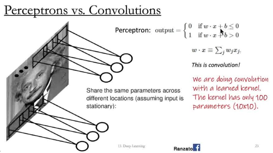
• Basically you're doing convolution but this time with dynamically learnt weights of the kernels / filters s.t. they are effective for the task
• We can even take multiple NNs, each to learn 1 kernel / filter.
• Since it samples by neighborhood, the input and output remain as 2D (rather than reshaped to 1D vector)
  • Output is called feature map
  • If there are multiple filters, we get multiple feature maps;
    • Each map is thus a channel of the output

Pooling

• Pooling: CNNs also aggregate response of a neighborhood (e.g. 2x2 patches)
  • Kind of like "downsampling"
  • But instead we do like max pooling
  • i.e. take a maximum within a neighborhood

Rectified Linear Unit

• In CNN the activation function, ReLU for short, is as follows:
  • f(x) = max(0, x)
  • this is a non-linear function
  • Thus it's called "non-linearity"

Convolutional Neural Network

• Each system: Input -> Convolution -> ReLU -> max pooling -> output

• Can be a bit flexible e.g. conv -> relu -> conv

  • You see some visualization on CS 231n
  • LeNet

• These systems are "Stacked" so the input goes through system after system

• Neural network is really just putting these things in a cascade

• Interleaving convolutions and pooling cause later convolutions to capture a larger fraction of the resultant image with the same kernel size

• Set of image pixels that an intermediate output pixel depends on = receptive field

• Local interactions - receptive fields

  • Assume that in an image, we care about "local neighborhoods" only for a particular neural network layer
  • Composition of layers will expand local to global

• Param sharing (which is already being done)

  • Since same weights applied to each neighborhood; equivariant representation regardless of location

Applications

• Image Classification
• Object Detection
  • Classifying objects and localizing them with a bounding box
• Semantic Segmentation
  • Associating each pixel in the image with a class label
• Instance segmentation
  • Associating each pixel in the image with the object to which it belongs