CS3244 Machine Learning

Collaborative & AutoML
- Trusted data sharing, tweaking params
Learning Element
- Which components are to be learnt
- How to represent the data & the components
- What feedback is available
- Main goal of the model
- Supervised learning: answer is provided
  - Learning an unknown function (focus of the module) that best fits answer
- Unsupervised learning: no answer provided
- Reinforcement learning: rewards provided
Concept Learning (Simplified ML)
- Search through hypothesis space for a consistent hypothesis
- Concept: boolean-value f(x) we want to learn
- Infer unknown boolean value function
- Training sample: row
  - Input Instance (X): comprises of Input Attributes (Features)
    - Input Attributes: Categorical variables
  - Boolean Output Attribute (Target): Y/N, 1/0, +ve/-ve
- Hypothesis: Conjunction of constraints on input attr
  - Think of this as a firewall filter
  - For every Input attr: X = specified_categorical_val, X=? (don't care), X=null
  - Input Instance satisfies (all constraints of) hypothesis if h(x) = 1
  - Expressive power (scope) vs hypothesis space (search space)
    - e.g. y = mx + c vs y = ax^2 + mx + c
    - More expressive model: more time & data to train
  - Hypothesis Space: Set of hypothesis
Goal: Find hypothesis that is consistent with noise-free training sample.
- Consistent = $\forall$ training instances, h(x) = 1 iff +ve instance, h(x) = 0 iff -ve instance
- Syntactically distinct Each feature gets "?" and "nullset" added to their domain
- Semantically distinct: Each feature gets "?" added to their domain, and one instance for the empty set (Φ).
- Exploit Structure: (h1(x)=1)->(h2(x)=1)
- More general or equal: $\geq_g$ , $\gt_g$
  - Partial order: reflexive, antisymmetric, transitive
Find-S algorithm:
- Start with most specific hypothesis (all null)
- When it wrongly classifies a +ve as -ve, minimally generalize it to satisfy input instance.
- Resultant hypothesis is a hypothesis in the Specific Boundary (summary of +ve training examples).
  - As long as the hypothesis space contains a hypothesis that describes the true target concept, and the training data contains no errors, ignoring negative examples does not cause to any problem.
  - Limitations:
    - Can't tell if Find-S found the target concept
    - Can't tell if training examples are noisy
    - Picks a maximally specific hypothesis (may not be unique)
Version Space w.r.t. hyp. space H and training examples D ( $VS_{H,D}$ )
- Subset of hypotheses from H that are consistent with D
- A large enough D can reduce $VS_{H,D}$ to just 1 hypothesis
List-then-eliminate
- Init as H, then reduce it to $VS_{H,D}$ by enumerating D, removing $h$ where $h(x)\neq c(x)$ . This results in the general boundary.
- Limitation: expensive to enumerate
Version space representation theorem (VSRT):
- Specific boundary S: set of most specific members of H consistent with D. (summary of +ve training examples; s(x)=1 -> h(x)=1)
- General Boundary G: Set of the most general members of H consistent with D. (summary of -ve training examples; ; g(x)=0 -> h(x)=0)
- Every consistent hypothesis lies on the path between S and G (inclusive) (S19, showing all consistent hypothesis)
Candidate-elimination algorithm
- G (most general set) = {(all wildcard)}, S (most specific set)= {(all null)}.
- Think of it as "or"ing any new clauses
- +ve Training example d:
  - If a hypothesis in S doesn't satisfy d, remove it, then add its least generalized versions (most attr changed, but minimal wildcards) h s.t.:
    - h satisfies d
    - h is less general than at least 1 h in G
  - Remove any hypothesis from G that doesn't satisfy d
- -ve Training example d:
  - Remove any hypothesis from S that satisfies d
  - If a hypothesis in G satisfies d, remove it, then add every least specialized hypothesis (fewest attributes changed) s.t.:
    - h doesn't satisfy d
    - h is more general than at least 1 h in S
- Limitations:
  - Noisy data (S & G will both fit to null)
  - Not enough data (insufficiently expressive hypothesis expression)
- Active Learner: should try to actively halve the search space; requires at least $log_2(VS_{H,D})$ examples to find target concept
Unbiased Hypothesis Space
- Must be Power set of training instance space ( $H = 2^x, |H| = 2^{|x|}$ , where $|x|=$ # of training instances)
  - $\forall$ training instance, if it is in the subset that the hypothesis represents, then h(x) = 1, else 0.
  - Hence, since T/F for every training instance, there are $2^{|x|}$ possible permutations of h(x)
- Change representation of S and G:
  - Every training instance is a variable (x1,1), (x2,0), (x3,0), ..., (xn, 0/1)
  - S is now (x1 v x4 v x5) all positive instances
  - G is now ( $\neg$ (x2 v x3)) all the negative instances
  - Need examples for every input instance in X to converge to target concept
- Limitation: Cannot generalize (predict unobserved) beyond training examples
Inductive bias assumpion
- Hypothesis found from sufficiently large training set also applies to unobserved data
Summarize data: save time & space
- Formally: given learning algo L, input instances X, target concept c, noise-free examples $D_c = {\langle(x_k, c(x_k)\rangl ...}$
  - Inductive bias of L is the minimal set of assumptions (B) s.t. (B and examples and any instance) is correctly classified
  - $\forall x\in X (B\wedge D_c \wedge x) \vdash (c(x) = L(x,D_c))$
  - Deductive Inference: If you have this set of assumptions, then L is provably correct (shown it correctly classifies everything)
  - Inductive Inference: The assumptions B may not hold, and thus L is not provably correct (relies on spamming data to work)
  - Basically 2 types of systems: one is inference system (we make few/no assumptions and it is not proven correct), one is deductive system (data fed in + assumption holds, proven correct classification)
  - Stronger assumptions allow you to make bigger guesses (classify more unobserved examples)
Inductive Bias of Candidate-Elimination: $B={c\in H}$
- Assumption for it to be provably correct: Target concept lies in hypothesis space
Learners w/ different inductive biases
- Rote-learner: classify input instances if previously observed, otherwise return null.
  - No inductive bias.
- Candidate-Elimination: Inductive bias $c\in H$
  - Find-S: $c\in H$ and all instances are only +ve if it is implied (i.e. noise-free & max. specific hypothesis classifies the instance as +ve)
Decision Tree (DT) Learning
- Represent hypotheses as a decision tree
  - Leaf: Classification
  - Internal Node: Test (attribute-value tests, bool decisions)
  - Edge: Decision Result
- Prefer to find compact decision trees (short height) to avoid creating 1 to 1 decision paths to the training examples & overfitting
- Can be represented as a boolean truth table to calculate the number of possible input instances:
  - m input attributes (boolean decisions)
  - $2^m$ possible paths
  - boolean target concept: 1 if the path is included
  - Hence $2^{2^m}$
- Expressive Power: SAT format $(\neg A \wedge B) \vee (A \wedge \neg B)$
- Algorithm:Recursive. Find small tree consistent w/ training examples
  - Greedily choose attribute (as the root of subtree) that results in the best segregation of +ve and -ve attributes by category
    - Most important: after splitting current set of examples using attribute, we have more subsets that fulfil base case
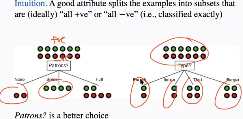
    - To evaluate the effectiveness of the split, information theory is applied to measure uncertainty in each category:
      - Entrophy measures uncertainty of RV target concept C (which has k possible values)
      - $H(C)=-\sum_{i=1}^{k} P\left(c_{i}\right) \log _{2} P\left(c_{i}\right)$
        Where P is proportion of examples with label $c_i$
      - For +ve/-ve cases, k = 2:
        For every category under the attribute: $B(q)=-\left(q \log _{2} q+(1-q) \log _{2}(1-q)\right)$
        Entropy is 1 when +ve/-ve are exactly the same # (p/(p+n) = 1/2), 0 when p/(p+n) = 0 or 1
        Entropy at a specific node H(C): $B\left(\frac{+ve}{+ve + -ve}\right)$
        Entropy of subnodes after A is used to split H(C|A):
        $H(C \mid A)=\sum_{i=1}^{d} \frac{p_{i}+n_{i}}{p+n} B\left(\frac{p_{i}}{p_{i}+n_{i}}\right)$
        Sum the entropy of every subnode multiplied by its proportion
        Information gain Gain(C, A) if attribute is used to split: expected entropy at the current node - expected remaining entropy
        $\operatorname{Gain}(C, A)=B\left(\frac{p}{p+n}\right)-H(C \mid A)$
  - Base cases:
    - If all examples in the tree are +ve/-ve, just return +ve/-ve
    - If no more examples down the tree (i.e. current example was not observed):
      - Plurality-value: majority voting amongst the set of examples along your path (tie-break randomly)
    - OR attributes is empty (examined all attributes but there are examples with different output): Use plurality value. Possibilities:
      - Due to error / noise
      - Stochastic distribution
      - Have not observed the attribute that distinguishes the examples
  - Whenever you go down the tree, you're always look at the next attribute
    - Chosen attribute used to split the examples set:
- Disjunctive normal form: ORing all the possible paths to +ve examples (19:00)
- Comparison w/ Concept Learning
  - Target concept: can be discrete (not binary like concept learning)
  - Training data: Robust to noise
  - Looks at all training examples
  - Hypothesis Space (complete, expressive)
    - VS concept learning's hardcoded assumption / hard bias (i.e. $c\in H$ )
  - Search strategy: Incomplete (only 1 hypothesis, soft bias; cannot estimate accuracy)
    - vS concept learning's complete version space (version space)
    - Refines search using all examples
      - VS concept learning's 1 example at a time
    - No backtracking
    - Structure: Simple to complex
      - VS concept learning's General to specific
  - Training instances same as Concept learning: boolean, discrete (categorical) and "continuous" (actually binned into categories by value range; can omit lower / upper bound)
Inductive bias of decision-tree-learning
- Shorter trees are preferred (e.g. its an approximation of breadth-first search using the most important attribute heuristic)
Occam's Razor: Short hypotheses preferred
- Simple hypothesis that fits data unlikely to be coincidence
- Many (non-meaningful) ways to define small sets of hypotheses
  - How do you know this small set is more relevant than any other?
Overfitting
- h overfits set D of training examples iff, given another h',
  - h's prediction error using set D (training error) < h'
  - but h' prediction error using test set is < h
  - Avoid overfitting:
    - Don't grow DT when expanding a node is not going to significantly improve prediction
    - Allow DT to grow and overfit data, then post-prune (the focus). Post-pruning techniques:
    - 1 Reduced-Error Pruning
      - Select by measuring performance over training & validation sets
      - 1 Partition data into training and validation sets
      - 2 Prune each possible node (remove subtree)
      - 3 Evaluate performance of this DT on validation set using plurality-value etc
      - 4 Greedily remove the one that most improves validation set accuracy
      - This produces the smallest version of most accurate subtree
    - 2 Rule Post-Pruning
      - Convert learned DT into a set of rules, each rule is the path from the root to a leaf (x=1 /\ y=2 /\ z=3) -> value = yes
      - Prune (generalize) each rule by removing any precondition that improves estimated accuracy
      - Sort pruned rules by estimated accuracy
      - Pros:
      - You can prune each path separately
      - Order of attributes not important
      - Easier to interpret
- Techniques:
  - Continuous-Valued Attributes: convert into discrete-valued using ranges
  - Attributes with many values (e.g. many unique dates):
    - GainRatio(C,A): Gain(C,A) / SplitInfo(C,A)
    - SplitInfo(C,A): $-\sum_{i=1}^{d} \frac{\left|E_{i}\right|}{|E|} \log _{2} \frac{\left|E_{i}\right|}{|E|}$
      - $|E_i|$ : elements in subnode w/ value i, $|E|$ : total elements
      - How uniformly does attribute A split examples; if $|E_i|$ is consistently very small, SplitInfo will be very large
      - Discourage selection of attributes w/ many uniformly distributed values
    - GainRatio usually used only if Gain is above a threshold (because if $|E_i|$ and $|E|$ is very close, SplitInfo blows up)
Theorems & Definitions
- Hypothesis $h\in H$ : Conjunction of constraints on input attributes
- Hypothesis space H: Set of single possible hypothesis
- Input instance $x\in X$ : Each data entry w/o the target value
- Training set D: set of -ve/+ve input instances
- Target concept c: The theoretical "ideal" hypothesis we want to arrive at to correctly classify every possible input instance of D (and of those unobserved)
- h(x): 0 (-ve) or 1 (+ve) classification of x based on h
- x Satisfies h iff h(x) = 1
- h Consistent with D: $h(x) = c(x) \forall <x,c(x)> \in D$
  - Every +ve training instance satisfies h
  - Every -ve training instance doesn't satisfy h
- Inductive Learning Assmptn: Any hypothesis that can approximate the target f(x) well over a large set of training examples can also approx. the f(x) over other unobserved examples
- General: h1 more general than or equal to h2 (h1 $\geq_g$ h2) iff any input instance x that satisfies h2 also satisfies h1:
  - $\forall x \in X\left(h_{k}(x)=1\right) \rightarrow\left(h_{j}(x)=1\right)$
- Specific: Inverse of general: h1 $\lt_g$ h2 = h1 more specific than h2
- Prop. 1: h consistent w/ D iff h(x)=1 when c(x)=1 and h(x)=0 when c(x)=0
- Prop. 2: If $c\in H$ , then final hypothesis of Find-S is consistent with D
- Version Space $VS_{H,D}$ : Subset of hypotheses $\in$ H that is consistent with D
  - Represents uncertainty of what target concept is
  - If $c\in H$ D is sufficiently large, can reduce $VS_{H,D}$ to {c}
  - Compact Representation: 2 boundaries:
  - (G)eneral bound: set of max general h consistent w/ D
    - $G=\{g \in H g$ consistent with $D \wedge(\neg \exists g^{\prime} \in H g^{\prime}>_{g} g \wedge g$ consistent with $D)\}$
    - there doesn't exist another hypothesis that is more general than g
  - (S)pecific bound: set of max specific h consistent w/ D
    - $S=\{s \in H \mid s$ consistent with $D \wedge(\neg \exists s^{\prime} \in H s>_{g} s^{\prime} \wedge s'$ consistent with $D)\}$
    - there doesn't exist another hypothesis that is more specific than s
- Version Space Representation Theorem: $V S_{H, D}=\{h \in H \exists s \in S \exists g \in G g \geq_{\mathrm{g}} h \geq_{\mathrm{g}} s\}$
- Easy proof structure:
  - Choose arbitrary $g \in G, s \in S, h \in H$ s.t. $g \geq_{\mathrm{g}} h \geq_{\mathrm{g}} s$
- Prop. 3: An input instance x satisfies every h in $V S_{H, D}$ iff x satisfies every member of S.