AI Planning (CS4246, Reinforcement Learning)
My notes for CS4246
Last Update: 2020
Bellman Equation
- Apply concept of dynamic programming and optimal substructure to do policy evaluation
R(s):
- Value of a state = its value + (Exploration Factor) x best value of next state
- How to get best value of next state?
- By choosing best action: the action that maximizes expected next state value
- Given (s, a), an action has the value of the sum of (value of next states) x (probability of reaching them).
- By choosing best action: the action that maximizes expected next state value
- How to get best value of next state?
| Var | Descript |
|---|---|
| s | Any possible state |
| s' | Any possible next state from s |
| a | Any possible action at s |
| V(s) | Value of s |
| R(s) | Reward of s (for staying on it) |
| A(s) | All possible actions at state s |
| γ | Exploration Factor |
| P(s'|s,a) | Probability of s' given (s, a) |
Bellman Equation Variants
R(s,a,s'):
- Reward for transiting from s to s' via a
- Choose the action that has gives the highest (transition reward + discounted future value of that next state)
R(s,a):
- Reward for taking action a at state s
- Choose the action that has gives the (highest reward + discounted value of all possible next states using said action)
Converting between reward functions
R(s,a,s') -> R(s,a):
- The reward for taking an action is the sum of (all its possible transitions) x (related transition rewards)
R(s,a) -> R(s):
- s' is abstracted out to "post(s,a)", which refers to the "post-state" for every (s,a). In this R:
// (s,a) always goes to post(s,a)
T'(s,a,post(s,a)) = 1
// The probability is factored in here
T'(post(s,a),b,s') = T(s,a,s')
// The states themselves don't have rewards
R'(s) = 0
// The reward for taking the action is put into the pseudo "post-state"
R'(post(s,a)) = gamma^(-1/2)R(s,a)
gamma' = gamma^(1/2)
Value Iteration Algorithm
- Repeatedly update the Utility function U(s) with [bellman update].
- U is only updated after every single state has been looped through.
// Returns Utility function U(s)
function Value-Iteration(mdp, err_threshold)
    loop:
        U_t = U_t+1, max_delta = 0
        for all states s in S:
            Update U_t+1 with bellman equation.
            Update max_delta if abs(U(s) - U_t+1(s)) exceed max_delta
        break loop if max_delta less than err_threshold(1-gamma)/gamma
    return U_t
Policy Evaluation Algorithm
- Same as Value Iteration.
- But we want to evaluate a given policy pi_i. Thus, we don't need to take the max, we just need to use the policy.
- Hence: Instead of taking the best action, take the action based on the policy
Policy Iteration Algorithm
- We don't need to calculate U(s) so accurately if we just want to find the optimal policy
- Two step approach:
- Init: Start with initial policy pi_0
- Policy Evaluation: Calculate Utility function U_i given current policy. See Policy Evaluation above.
- Policy Improvement: Calculate new policy pi_i+1 using U_i.
- Termination: Repeat until the new and old policy are the same (no change).
// Returns policy pi
function Policy-Iteration(mdp)
    U = set all to 0
    pi = random policy
    loop
        unchanged = true
        U_i = Policy-Evaluation(pi, U, mdp)
        for all states s in S:
            If the best action at s is different from pi[s]:
                Update pi[s]
                unchanged = false
        break if unchanged
    return pi
The check for the best action is done as follows:
- Identify the action with highest utility at s
- Check if it is the same action taken in the policy
Modified Policy Iteration
- Only do k iterations (i.e. up to a horizon) instead of until no change
Types of tasks in RL
- Prediction: Given a policy, measure how well it performs.
- Control: Policy not fixed, find optimal policy.
- See this StackExchange post
Model-Based Prediction
- Prediction: Given traces of a policy and the final reward, learn the utility function (based on policy) by constructing the model from the data using an agent:
- Learn transition model and reward function using an Adaptive Dynamic Programming (ADP) agent.
- Calculate the Utility function.
// persistent variables
s_prev
pi: policy
mdp: current constructed model, rewards and discount
U: table of utilities
Nsa: Table keeping count of number of times at state s, action a was taken
Nsas': Table keeping count of number of times the next state was s' given (s,a) (thus s,a,s')

// Called everytime a new percept is observed by the agent
// Percept: (previous state s, current state s', current reward r')
function PASSIVE-ADP-AGENT(percept)
    // Initialize U[s] and R[s] with its observed reward
    if s_curr is new:
        U[s_curr] = r_curr
        R[s_curr] = r_curr

    // If the state was arrived from a transition, update the transition function
    if s_prev not null:
        // Increment # of times event happened
        Nsa[s_prev,a]++
        Ns'sa[s_curr,s_prev,a]++

        // Update transition function for every known reachable state by (s,a)
        for every state where Ns'sa[state,s,a] > 0:
            // Update probability of transition
            T(s,a,s') = Ns'as[s,a,s'] / Nsa[s,a]

    // Update U based on new transition function
    U = Policy-Evaluation(pi, U, mdp)

    // If the policy is terminal, then don't recommend new actions
    if s_curr is terminal:  s_prev,a = null
    else:                   s_prev,a = s_curr, pi[s_curr]
    return a
Model-Based Control
- Learn the policy, not the utility
- Just replace Policy-Evaluation with Policy-Iteration
- The policy no longer stays fixed but changes as transitions and rewards learnt
- Note that however the algorithm is greedy and may not return the optimal value
-greedy
- Hence must do e-greedy exploration (choose a greedy action with 1-e probability and random action with e probability)
- Greedy in the Limit of Infinite Exploration (GLIE), e = 1/t
- Start with a high epsilon, then slowly reduce the number of random actions you take (by reducing the value of e) with every policy iteration as you become more and more certain you have an optimal algorithm
Monte Carlo Learning
- Monte Carlo Learning (Direct Utility Estimation)
- Given a series of states as a "trial" e.g. this is a trial: (1)-.04->(2)-.04->(2)-.04->(3)-.04->(4)-.04...->(5)+1
- Keep a running reward average for every state; after infinite trials, sample average will converge to expected value
- e.g. for the above trial, maybe state (1) has a sample total reward of 0.72
- Calculate by taking sum of rewards from that state to the end)
- If a state is visited multiple times in a trial e.g. state (2):
- first-visit: take the sum of rewards from only on the first visit per trial
- every visit: take multiple sums for every time the state was visited in a trial.
- e.g. for the above trial, maybe state (1) has a sample total reward of 0.72
Assume state s encountered k times with k returns, and each summed reward is stored in G_i(s).
- Note that G_i(s), given infinitely many i iterations, will converge to the true value; hence G_i(s) - U_k-1(s) is the MC error, or prediction error
- The difference between the current U_k(s) and the previous U(s) is the prediction error (if you want to mnimize absolute loss, you can use median instead of average)
- Note that U(s) here can also apply to U(s,a), and can also be renamed as Q(s) and Q(s,a)
# Calculating "value sum": Sum the values from s to the end in the trial

# Monte Carlo Prediction (Learning U(s))
After every trial:
    Take every state (or first state occurence) and calculate its value sum
    Increment Ns
    # Update U(s) after every trial
    U_k(s) = U_k-1(s) + 1/k(sum - U_k-1(s))

# Monte Carlo Control (Learning pi)
After every trial:
    Take every (s,a):
        newR(s,a) = take every/1st (s,a) and calculate its value sum
        Increment Ns
        # Update Q(s) after every trial
        Q(s,a) = Q_k-1(s,a) + 1/k(newR(s,a) - Q_k-1(s,a))
    For every s:
        pi(s) = Take action that maximizes Q(s,a)
Advantages
- Simple
- Unbiased estimate
Disadvantages
- Must wait until a full trial is done in order to perform learning
- High variance (reward is the sum of many rewards along the trial), so need many trials to get it right
Temporal Difference Learning
- i.e. TD(0)
- Very similar to Monte Carlo Learning
- Replace the prediction error with the temporal difference error
Transition from state s to s'.
Alpha is the learning rate.
- Converges if alpha decreases with the number of times the state has been visited (think GLIE)
: Temporal Difference target
- Reward of current state + Expected utility from the new state s'
- If there is no error, this should be equal to the current utility
- this is basically bellman update, policy evaluation
: Temporal Difference error
- (amount of utility change from previous state s to current state s')
- difference between the estimated reward at any given state or time step and the actual reward received
- Reward of current state + discounted future reward(future state) - expectedRewardWithIncludesFutureRewards(s)
## Prediction
TD-Agent:
for every percept (curr_state s', immediate reward r')
if s' is new:
    U[s'] = r'
if s not null:
    Ns[s]++
    # Note that alpha is a function that takes in Ns[s]
    # It steadily decreases over # of iterations
    U[s] = U[s] + alpha(Ns[s])*(r+gamma*U[s']-U[s])
if s' terminal:
    s,a,r = null
#else: # update prev data
    s,a,r = s',pi[s'],r'
return a
Advantages
- Can learn with every step (in a trial)
- Usually converges faster in practice
Disadvantages
- Online; lower variance, but estimate on how good your estimate is; biased
- Assumes MDP
- Error can go in any direction
SARSA
SARSA uses TD learning w.r.t. a specific policy:
On-policy
Q-Learning
Q-Learning uses TD learning w.r.t. the optimal policy (s' is the next state after (s,a) is taken):
Off-policy
n-step TD
Alister Reis has written a very good blog post on this
- n-step: n is the # of steps you use in your temporal difference.
- 1-step (or ):
- : Temporal Difference target
- : Temporal Difference error
- 2-step (or ):
- : Temporal Difference target
- : Temporal Difference error
- s: the state you stepped into, R(s) is the reward for that state, s' and s'' are s_t+1 and s_t+2 respectively in that trial
- The reason why gamma stacks is because it is multiplicatively stacked with every iteration (think of it as "unpacking" U(s))
- 3-step and beyond is just continued "unpacking"
- 1-step (or ):
TD()
Alister Reis has written a very good blog post on this
- Basically you want to do n-step but you don't want to choose n
- i.e. instead of calculating n-step return , you want to calculate
- So you take a and use it to multiplicatively weight all the
- i.e.
- If you remember your geom progression,
- So to normalize all this to 1, we need to multiply it by
- We get this cursed formula
- Which is equal to
- Now you're probably wondering how to calculate this without calculating to the end
- Because I know I was wondering about it since my prof didn't talk about it
- So that's why some geniuses used something called eligibility trace which keeps track of how "fresh" each state is (based on frequency and last visit) (img src).
- Since it sums to infinity (or at least, sums to the end of the trial), They use this eligibility trace to iteratively calculate with each timestep as opposed to calculating it all in 1 shot at the end

- i.e. every state has an eligibility trace, init at 0
- when state is visited at that timestep, its adds 1
- This is called an accumulating eligibility trace.
- If just reset to 1, it's called a replacing eligibility trace.
- at every timestep these values are multiplied by lambda and gamma (they "deteriorate")
- With this eligibility trace system, you no longer just update the U(s) of 1 state with every timestep, you run the update for every state, but the TD error is weighted by each state's own eligibility trace.
- So for every timestep, update all eligibility traces:
eligibility *= lamb * gammaeligibility[state] += 1.0
- Then get the TD error for the current timestep:
td_error = reward + gamma * state_values[new_state] - state_values[state] - Then finally update U(s) for all states:
state_values = state_values + alpha * td_error * eligibility - As per Alister
- So for every timestep, update all eligibility traces:
See also?
On & Off Policy
- On-policy:
- One policy used for both generating data & training
- e.g. SARSA
- Converges to optimal policy if:
- Off-policy:
- One behavior policy for generating training data
- generating data: interacting with environment to get info
- One target policy to be trained
- Converges to optimal policy if:
- Decaying
- Every transition is taken infinitely many times in behavior policy
- Converges to optimal policy if:
- One behavior policy for generating training data
Function Approximation
- State space too large -> solve by approximating utility function
- Approximate using a linear function of features
- Define a linear function to approximate U(s):
-
- e.g.
- s in this case is (x,y)
- And in this linear function you have a vector of parameters =
- Goal is to learn
Supervised learning
- Method 1: learn using set of training samples
- Given a set of training samples beforehand
- Do least squares estimation to fit params
- e.g. given linear function
- you have a set of samples where U is value of the linear function and x and y are the function input
- you can do linear regression to solve
Online learning
Method 2: learn on the job
Gradient descent using every piece of evidence
For every parameter in :
- , which expands to:
- , which expands to:
e.g. given linear function
We can extend the param formula to temporal difference learning for TD:
As well as Q-learning:
These are called semi-gradient methods because target is not true value but also depends on θ.
Sources of instability
- Instability and divergence tend to arise when the following three elements are combined:
- Function approximation
- Bootstrapping
- Off-policy training
- Training on transitions other than that produced by the target policy.
Deep Q-learning
- Online Q-learning with non-linear function approximators is unstable
- DQN uses experience replay with fixed Q-targets:
- Makes input less correlated, reduce instability
- Procedure:
- Take action using ϵ-greedy
- Store the observed transition in a round-robin buffer
- When there are enough transitions:
- Sample random mini-batch of transitions from buffer
- Set targets to
- Gradient step on mini-batch squared loss w.r.t.
- Set to every C steps
- Get more transitions & repeat
- Haha if you didn't get that don't worry I don't think I'd get it if I didn't use Google gdi fucking useless slides
Policy Search
- Often use the Q-function parameterized by to represent the policy:
- Adjust to improve policy
- However, the max operator makes gradient based search difficult.
- Thus, represent the next state as a vector of probabilities at state s, given action a (i.e. ) using softmax:
- With this vector of probabilities we want to maximize of w.r.t .
- We can do this by differentiating w.r.t. , then taking a gradient ascent in that direction.
- This "direction" is the policy gradient vector represented as
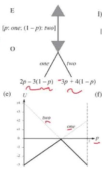
TD(0) example where only 1 step is taken:
- You're at state and returns vector of action probabilities
- Recall = reward of action x action probability
- Thus policy gradient vector
If considering more steps, calculating the policy gradient becomes:
- : Trajectory generated by policy
- : Probability policy generates
- : sum of rewards from trajectory
- Using the policy gradient theorem, this can be written as:
- is probability of being in state s (at any point in time) given initial state and
- formal: = is the stationary distribution of states under (Sutton)
- is probability of being in state s (at any point in time) given initial state and
Proof of Policy gradient theorem:
- Computing the gradient of the value of the policy at state s:
- We can expand the equation using product rule of calculus
- If we unroll the last term, we get this eqn:
- After repeated unrolling, where is the probability of transitioning from state s to state x in k steps under , we get this general eqn:
- Taking expectation over the initial state distribution (?) we get
REINFORCE algorithm
- Monte Carlo approximation of the advantage function (?)
- Continuing on, we can approximate the policy gradient using
- Thus at each step j, we can update the params by taking its prev value + (learning rate) x (reward at step) x (rate of change of w.r.t. ) / ())
- : learning rate
- : reward at step j
- Differentiating the next state softmax vector w.r.t. the parameters
- We can use the dy/dx(ln(x)) identity to simplify it, thus obtaining the REINFORCE algorithm
Baseline
- In practice we can reduce the variance using any function .
- Recall that for the REINFORCE algorithm we are estimating
We can replace with , where is any function and it stays the same. That replaceable portion is called the Advantage function.
It stays the same because sums to 1 (since it's a vector of action probabilities). Since the derivative of a constant is 0, doesn't have any actual effect.
Modifying the Advantage function
- Monte Carlo estimate: Set
- TD(0) variant: Set and replace
- Thus, TD(0) variant:
- The parameter update function would then become:
- (?) I don't know how to derive this eqn lmao I only assume the advantage function or TD error is multiplicatively applied here
- We can extend this to n-step TD or TD() by replacing .
- We can also use a value function estimator with param to estimate the value. This would be called the actor-critic method, because:
- you're learning a policy (actor) managed by the params
- you're also learning a value function managed by params used only for evaluation (critic)
Partially Observable MDP
- Are you seeing a trend?
- Function estimation: action replaced with probability vector
- POMDP: So you're uncertain about current state?
- No problem, just replace state with probability vector belief =
- Filtering: Tracking
- No problem, just replace state with probability vector belief =
Updating The Belief
- This is defined as :
- b: belief, a: action, e: evidence
- Next belief based on evidence observed given (b,a)
- C: normalizing constant to make belief sum to 1
- : Probability of receiving evidence upon entering
- Given bae, = (Pr. of seeing e at s') x (Pr. of action a bringing you to s' based on your previous states' likelihood)
- If small state space, just need to use optimal policy to map belief to action.
Reward Function of Belief
Expected reward of a belief: sum of R(s) x every probability
This is equivalent to a dot product of b(s) and R(s)
Extending this concept to the utility of a belief given a fixed conditional plan p from state s (i.e. )
- Optimal policy: choose action offering best utility
- Conditional plan: Think of it as if/elifs to return an action based on belief probabilities
Given an optimal policy, the Value function of a belief is the best action given said conditional plan and belief:
With |A| actions and |E| observations, there are distinct depth-d plans
However if we want to calculate the value function of a conditional plan:
if you don't understand don't worry I don't either so I'll simplify based on other info
The value of action, assuming the current state is s, = (reward of the current state) + discount x (expected value of the next state)
- Expected value of next state has so many factors now:
- Probability of transitioning to that state x
- Actual expected value of that state x
- Probability that you are actually at that state given the evidence you receive upon entering said state
- Expected value of next state has so many factors now:
You basically want to choose how far you want to look ahead (your depth / # of steps)
Then, calculate for every possible (s, action) pair, looking up to the chosen depth
Then, you can plot the hyperplanes (see below) s.t. given the probability of being in a state, when should I do which action s.t. I maximize my overall value
n step/depth plan
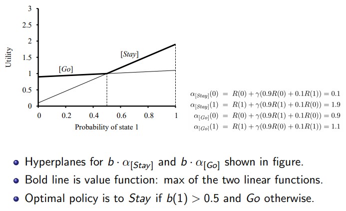
- Example: Simple boolean state world.
- R(0) = 0, R(1) = 1
- Actions: Stay Pr(0.9), Go Pr(0.9).
- Discount factor γ = 0.9
- Sensor reports correct state with prob 0.6.
- Agent should prefer state 1
Calculating the value function vectors:
0 step/depth plan literally don't do anything because 0 steps lmao got'em
1 step/depth plan:
- Value = Current state + next state
- Using this we can plot the hyperplanes (lines for probability)
- Then we always choose the highest line at any point (thus maximizing utility)
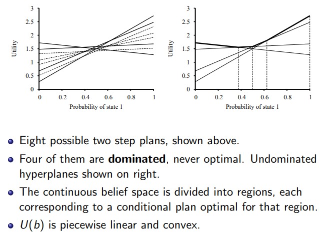
n step/depth plans
- The more steps you look ahead, the more refined U(b) becomes
- U(b) is convex
- Some hyperplanes are dominated (i.e. never max) so can ignore them
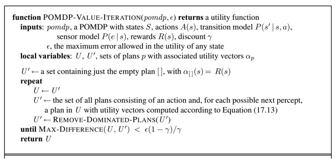
POMDP Value Iteration
- Just keep calculating plans, removing useless plans
- If no change after awhile then return U
- PSPACE-hard problem lmao
- Variant: SARSOP
Game Theory / Multi-agent
Single-move game
- 2 player games chosen for simplicity
- Strategic / Normal form: Payoff matrix:

- 2 players have their own utility based on their actions and the action of the other player
- Strategy: Policy
- Pure strat: deterministic
- Mixed strat: stochastic
- Strictly dominated: strategy s is always better than s' regardless of whatever strategies other players have
- Weakly dominated: strategy s is sometimes better than s'
- Strategy Profile: Each player assigned a policy
- Can be used to compute game's outcome
- A solution is a strat profile where all strats are rational (i.e. maximize their E[U])
- Rational strategy: maximize expected utility (regardless of other agents' possible actions)
- Iteratively remove dominated strategies (e.g. prisoner's dilemma, will always be better if testifying)
- How to evaluate a solution?
- out1 Pareto optimal: All players prefer outcome out1 (the best value regardless of actions)
- out1 Pareto dominates out2: All players prefer outcome out1
Equilibriums
- Testing for Equilibrium: Fix all except 1 strategy, see if changing the agent's strategy can improve his value
- Dominant Strategy Equilibrium: Each player have their dominant (best) strategy
Nash Equilibrium (local optimum): all all players can't get better outcomes from changing from their assigned strategies
- Test by fixing all policies except the player's policy
- Local optimum if a strategy involved is weakly dominated
Prisoner's dilemma example

- Rational choice for both: testify
- (testify, testify) Pareto dominated by (refuse, refuse)
- hence dilemma
Finding Pure Strategy Nash Equilibrium
- Go through every column and mark cell (for tht column) which has maximum payoff for row player
- Basically the same as testing for equilibrium; fix strategy and find best
- Go through every row and mark cell (for tht row) which was maximum payoff
- If both players agree on their optimal outcomes, that is a Pure Strategy Nash Equilibrium
Finding Mixed Strategy Nash Equilibrium
- This particular strategy doesn't always work
- Do the same as findiing pure strategy: fix the other agents' strategy, then choose your best strategy
- Optimal for row player: Assign fixed probabilities to the actions of row player, then calculate the expected payoff for each action of the column player
- Choose probabilities such that it doesn't matter what the column player does.

- Repeat for the other player to get the mixture
- Mixed solutions will always have at least 1 nash equilibrium
Finding 2 player 0-sum game solution
Sum of outcome (payoff) is 0
Follow the same concept as above; fix probabilities for one, then choose a strategy where the opponent's choice doesn't matter 
One player always positive outcome, the other player always negative outcome
Both players want to maximize / minimize
Minimax strategy gives a Nash Equilibrium
- https://staff.ul.ie/burkem/Teaching/gametheory2.pdf
- Page 3
- The first player assumes the 2nd player knows their strategy & will minimize their profit
- Assume the first player is the row player. Expected reward of row player:
- p = probability of row player taking left action
- q = probability of col player taking left action

- Find i.e. rate of change of reward w.r.t. enemy policy.
- We want this to be 0 i.e. row player strategy doesn't depend on col player's strategy.
- Differentiate eqn w.r.t. the enemy's probability q and get optimal row player probability.
- To calculate the expected value (iee. ), repeat the same procedure for the enemy; Differentiate eqn w.r.t p.
- If it's 0-sum, both players will reach the same probability value
- Partial Derivatives:
- https://staff.ul.ie/burkem/Teaching/gametheory2.pdf
- Given these expected outcomes w.r.t. p, choose p s.t. you maximize the minimum
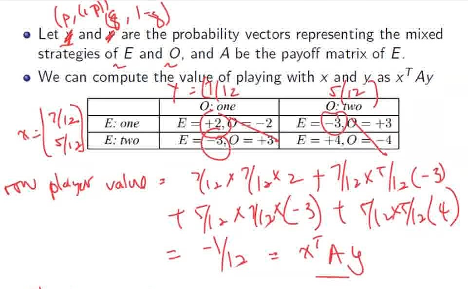
minimax:
- x: probability vector representing strategy of row player
- y: probability vector representing strategy of col player (which is just [0,1], [1,0] since it's a pure strat)
- (row player uses strategy represented by probability vector x) + best by col player = v (value)
- A: payoff matrix for the row player
- Linear programming solution:
- j: index of the column
- aij: cell of the payoff matrix A
- this is a nash eqiuilibrium
- pure strategy can be used (pure strat because the choices are discretizable even though the outcomes are based on opponent's probabilities

PPAD-complete: computationally hard even for 2 player games
Extensive form: game tree See 33:40 w12
- Modelling uncertainty: players have a chance to take random actions (and these edges have probabilities associated with them)
- Handling partial observability: define information sets
* **information set** = possible_current_nodes(previously_observed_actions)
* Imagine the game as a complete tree, where edge is an action and node is a state- information set is all the nodes you can possibly be at, given your observations of your initial state and what actions you observed happened
- https://en.wikipedia.org/wiki/Information_set_(game_theory)
sequential version / extensive form: look ahead and see best equilibrium based on 1st player subgame see 38:00
- every subgame must also be perfect equilibrium
repeated game:
face same choices but with history of all player's choices
backward induction:
- identify optimal solution for last solution
- identify previous solution that optimizes current solution and itself
- if reward indifferent to time, then it doesn't matter
cooperative equilibrium:
- equilibrium: once enter don't want to switch
- e.g. prisoner's game
- perpetual punishment: start with cooperate, then never cooperate if other betrays
- tit-for-tat: start with cooperate, then copy other player's previous move