CS4246 Cheatsheet
Problem Specification
- Initial State
- Possible Actions Action(s)
- Transition Model Result(s,a)
- Goal Test
- Path Cost c(s,a,s')
- Admissible Heuristic: Never overestimate cost to goal
- Consistent / Monotonic: Straight path (to goal) always shorter than a curved path.
- Factored Representation: State representeed as SAT
- Fluents: state variables in said representation
STRIPS
- Problem spec: Initial State, Actions, Result, Goal
- Action: Action(params),
- Precond: Descript
- Effect: Descript
- Negation (Delete list), otherwise Add List
- Goal: Partial state, must be fulfilled
- Action: Action(params),
- State: +ve literals ANDed together with no unknown variables or functions.
- Negation not allowed (use literals that are negative)
- If literal not specified in state, it is false (database semantics)
- Search:
- Forward: wk 1 39/65
- Backward: wk 1 40/65
- Relevant-state search:
- Actions are relevant when:
- Action doesn't negate a predicate in the current goal
- Action unifies a predicate in the current goal
- Add the preconditions of the action to current goal descript
- Actions are relevant when:
- Relevant-state search:
- Heuristics:
- Ignore preconditions
- Ignore delete lists
- Assume subgoal independence, decompose problem
- Turning into SAT problem
- Complete the initial state by adding negations to omitted ground literals
- Complete the goal by taking every possible grounded combination of the goal and ORing them together.
- e.g. ...
- Axioms
- successor-state:
- Solves Frame problem (most actions don't change fluents) 60/65
- Pre-condition: Action taken at time => Precondition was true
- Action Exclusion: both actions cannot be taken at same time step.
- Not (Action1 at t) v Not (Action2 at v)
- successor-state:
Utility Theory
- Axiomatic approach, assume agent has consistent preferences for outcomes (GT >, LT <, EQ ~). Represented as U(Outcome).
- Utility can be preserved with monotonically increasing transformation.
- Axioms
- Orderability / Completeness: For any 2 outcomes, only 1 preference (agent prefers one, or both equal)
- Transitivity: (A > B) /\ (B > C) => (A > C). Otherwise irrational
- Continuity: If 3 outcomes: A > B > C where B is sandwiched. Then there must be a p where agent always get B, then A with probability p or C with probability (1 - p).
- Lotteries: [p1, O1; p2, O2...] Probability p1 for outcome O1 etc
- Susbstitutability: If A ~ B, then they can be swapped within a lottery
- Monotonicity: If A > B, then agent must prefer A.
- Decomposibility: 16/52 Chained lotteries can be reduced to simpler ones
- Expectations:
- Expected U(outcome): All probabilities x outcomes
- Principle of Maximum Expected Utility (MEU)
- Rational agents must maximize expected utility
- Expected Monetary Value (EMV): wk1, 28/52
- Risk-neutral: montonically increasing, line up
- Risk-averse: Log of money amount.
- Risk-seeking: U(L) is more than the straight line later on
- Certainty Equivalent: Value agent will accept in lieu of a lottery
- Risk Premium: EMV - certainty equiv
- Normative theory: how agents should act
- Descriptive theory: how they actually act
- Irrationalities: Ambiguity aversion, framing effect, anchoring effect (35/52)
- Optimizer's curse: 36/52
- Bayesian and Decision networks 40/52
- Given observed outcomes, calculate probability of affected outcomes
- Chain rule
- calculate expected outcome value based on these probabilities
- Value of Perfect Information VPI
- Given this new information, calculate new expected outcome
- Split into cases (See 47/52)
- Pr(info success) x Pr(success)
- Pr(info fail) x Pr(fail)
- VPI = new outcome - old outcome
- Split into cases (See 47/52)
- Non-negative expected value
- Not additive with other VPIs
- Given this new information, calculate new expected outcome
MDP
Principle of Optimality: A value of a state is its reward + best future rewards from state. 20/54
Online Search 39/54
- Handling curse of dimensionality with MDPs
- Imagine it as a tree
- Nodes: values , Edges: transitions
- Tree size:
- Sparse Sampling: Don't check future for some states
- Rollout: Simulate many trajectories from a state to estimate action with best returns
- Monte Carlo Tree Search: 43/54
- Selection: Dig down the tree until depth reached or node not simulated yet
- GLIE. Explore first, then become more greedy (Decrease epsilon as time goes on).
- Expansion: If state not terminal, Create child nodes from this state.
- Simulation: Choose one of the child nodes,C, and do random rollout.
- Backpropagation: Propagate the reesult of the rollout to update node values from C to root.
- Selection: Dig down the tree until depth reached or node not simulated yet
- Upper Confidence Tree (UCT) 48/54
- A strategy for selecting a node for MCTS
- Choose action that optimizes (current estimate + exploration * sqrt(ln(times node visited) / ln(times node visited and took action a))
- Balance expected value and exploration
Bellman Eqn 21/54
Evaluate policy using dynamic programming
Value Evaluation: Init V = 0
:
:
:
- (s): state, (s,a): action, (s,a,s'): transition
Value Iteration: Given model (R, A, T(s,a,s')), recurse bellman until all converge
Policy Iteration: Init V = 0, = random
- Evaluate based on , not max (using bellman)
- Update if V for any action <
- Stop when no change / horizon reached
Prediction: Evaluate a given policy, Control: Find optimal policy
Model-Based, Adaptive Dynamic Programming Agent: Iteratively given observations, construct R and T(s,a,s'):
- R: = observed R(s). In addition, U(s) = R(s) when a new R(s) is observed
- T(s,a,s'): (times transition observed) / (times action at state)
- these variables are tracked with a table
- Prediction: Update U using Policy-Evaluation after each observation
- Control: Update U using Policy-Iteration after each observation
-greedy: action = (1-e)(best) and (e)(random)
Greedy in the Limit of Infinite Exploration (GLIE),
Monte Carlo Learning (Direct Utility Estimation): of rewards from s to end]
- = of rewards from s to end
- i-th episode, k episodes thus far
- Concept: [(New Info) - (Current Estimate)]
- New Info = Target, Difference = Error
- equals equals
- Monte Carlo Target:
- Monte Carlo Error (converges to 0 when k = ):
- Prediction: Calculating V(s) is enough
- Control: Calculate , then update by
- = of rewards from s to end
Temporal Difference Learning (TD(0)): Same as MC Learning but estimate with every step in the episode instead.
- Change the target:
- $ = V{k[j+1]}(s) = V{k[j]}(s) + \alpha(R{k[j+1]}(s) + \gamma V{k[j]}(s') - V_{k[j]}(s))$
- k episodes thus far, j-th step in the kth episode
- TD Target:
- Converges faster but biased
- SARSA: TD(0) using 1 for generating data and training(on-policy)
- State-action-reward-state-action: algo for learning MDP
- Future value estimate by action taken by
- Target:
- on-policy converges if -greedy
- Q-Learning: TD(0) using 2 : 1 for generating data, 1 training (off-policy)
- Future value estimate by best action based on current estimates
- Target:
- off-policy converges if decays and all transitions taken infinitely times
n-step TD (TD(n)): Somewhere between TD & MC: Change target to combine future steps in 1 update
- 0-step (): TD target =
- 1-step (): TD target =
- 2-step (): TD target =
TD(): n = , = 0 to 1, weight and normalize by geometric progression
- : New observed V(s) given n-step estimation
- Conceptually, All are estimations of the same thing, hence the eqn =
- Using Geom Progression:
- Hence
- Computation:
- Eligibility trace : track how "fresh" each state is by frequency and last visit
- Init = 0
- Types:
- Accumulating : += 1 if state visited at step
- Replacing : = 1 if state visited at step
- "Decaying Effect": With every timestep,
- Eligibility trace : track how "fresh" each state is by frequency and last visit
- Using eligibility traces, and timestep, update V(s). The TD error is weighted by each state's own eligibility trace.
- timestep, update all eligibility traces:
eligibility *= lambda * gammaeligibility[state] += 1.0
- Then get the TD error for the current timestep:
td_error = reward + gamma * state_values[new_state] - state_values[state] - Then finally update U(s) for all states:
state_values = state_values + alpha * td_error * eligibility
Function Approximation
- State space too large, approximate with a linear function that takes in a vector of params :
-
- Multi-variate s: , where s=(x,y)
- : Can approximate by:
- Keep a constant, then estimate using 1 linear fx per s
- Use a single linear fx that accepts s and a as params
- Supervised Learning
- Learn using initial training sample set
- Do least squares estimation to fit params
- e.g. given linear function
- you have a set of samples where V is value of the linear function and x and y are the function input, do linear regression to solve
- Online Learning
- Use gradient descent to minimize Error(s) (MC Error, TD Error etc) by modifying params on every observation
- Error(s) = (approximated_V(s)) - (observed_V(s))
- "approximated_V(s)" is
- observed_V(s) - approximated_V(s)
- : differentiate linear function w.r.t.
- You can swap out the error portion in the assignment above with any of these:
- Monte Carlo Error: (approximated_V(s)) - (observed_V(s))
- Semi-gradient methods (target biased as it depends on ):
- TD Error:
- Q-Learning "Error":
- Deadly Triad: Sources of instability
- Function Approximation
- Bootstrapping: Use current estimates as targets, e.g. TD Rather than complete returns, e.g. MC
- Off-policy: Training on transitions other than that produced by the target policy.
Deep Q-Learning: Q-learning with non-linear function approximation
- Use experience replay with fixed Q-targets to make inputs less correlated & reduce instability
- The procedure below uses double Q-learning
- Procedure:
- Take ϵ-greedy action using approximated policy from main policy_NN
- Store observed transition in a round-robin buffer
- Repeat until transitions, then loop times:
- Sample random mini-batch of transitions from buffer. Do the following as a batch:
- Compute based on actions policy_NN took to produce the transition
- Compute
- Compute by
- Compute Huber loss between and
- Gradient step on loss
- Increment episode count
- Set target_NN's params to main_NN's params after every C episodes
- Reset environment, update and repeat from step 1
Policy Search
- See other document.
POMDP
- Updating belief' given (b, a, e)
- Set initial belief (set of probabilities of being in each state)
- Do action: next_state, all Pr(you were in prev_state) x Pr(transit)
- Use evidence: state, x Pr(evidence seen at state)
- Normalize s.t. all state beliefs = 1
- Value () of plan with n steps
- Recursively "unpack" future rewards as necessary
- Evaluate E[value] after executing plan from
- Plan: Pre-planned sequence of steps
- Optimal Plan:
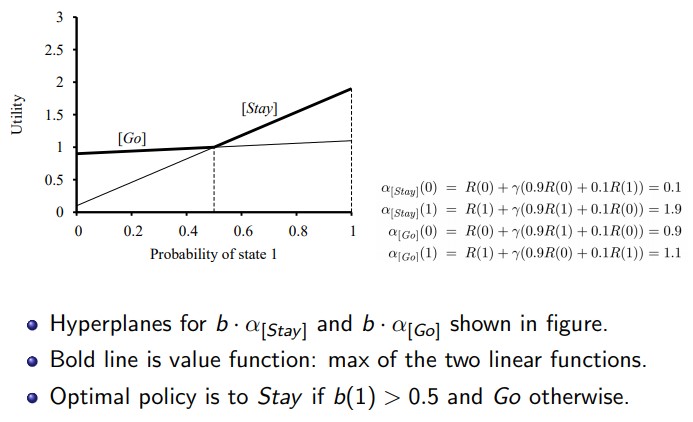
- x-axis: Pr() (0-1), y-axis: value )
- Plot: All possible values of plans w.r.t. Pr(s) (). Each plan is a line formed by 2 points:
- Point 1 at x-axis 0:
- Point 2 at x-axis 1:
- Optimal: Switch between plans that offers highest given regions of Pr()
- POMDP Value Iteration: Keep calculating plans while removing dominated plans. If no change after awhile, then return set of dominating plans.