
CS4268 Quantum Computing

Linear Alg

  • Basic Matrix Properties
    • Addition, must be same size:
      • Commutative: A + B = B + A
      • Associative: A + (B + C) = (A + B) + C
    • Multiplication:
      • NOT Commutative
      • Associative: A(BC) = (AB)C
      • Distributive 1: A(B + C) = AB + AC
      • Distributive 2: (A + B)C = AC + BC
  • Shorthands: i = Row index. j = Col index.
  • Invertible: A(A1)A(A^{-1}) = (A1)A(A^{-1})A = InI_n. Only square matrices can be invertible
    • Inverse is unique
    • Nonsingular: Determinant \neq 0
    • Prata: (AB)1=B1A1(AB)^{-1} = B^{-1}A^{-1}; likewise, (AB)=BA(AB)^{*} = B^{*}A^{*}
    • No mercy to lonely: (kA)1=k1A1(kA)^{-1} = k^{-1}A^{-1}
    • 360 no-scope: (A1)1=A(A^-1)^{-1} = A
    • Transpose's kyōdai: (AT)1=(A1)T(A^T)^{-1} = (A^{-1})^{T}
  • Transpose
    • Addition: (A+B)T=AT+BT(A+B)^T = A^T + B^T (no diff)
    • Prata: (AB)T=BTAT(AB)^{T} = B^{T}A^{T}
    • Spares the lonely: (kA)T=kAT(kA)^{T} = kA^{T}
    • 360 no-scope: (AT)T=A(A^T)^{T} = A
    • Invert's kyōdai: (AT)1=(A1)T(A^T)^{-1} = (A^{-1})^{T}
  • Trace of square matrix M Tr(M)Tr(M): sum of its diagonal elements.
  • Dot product: rowcol=i=1nrowicolirow\cdot col = \sum_{i=1}^{n}row_icol_i
    • For 2 vectors, Inner product is the (scalar) result of the dot product
    • For 2 matrices, Inner product is <A,B>=Tr(AB)< A,B > = Tr(A^{\dagger} \cdot B)
  • Matrix Multiplication: cij=kn=aikbkjc_{ij} = \sum_{k}^n = a_{ik}b_{kj}
  • v1||v||_1 = 1-norm = maxj(i=1naij)\max_j(\sum_{i=1}^n|a_{ij}|)
  • v2||v||_2 = 2-norm / Euclidean norm = i=1nj=1naij2\sqrt{\sum_{i=1}^n\sum_{j=1}^n|a_{ij}|^2}
  • Complex number: a+bi,i=1,i2=1a + bi, i=\sqrt{-1}, i^2=-1
    • Multiplication: (x+yi)(u+vi) = (xu-yv)(xv+yu)i
    • Norm: v22=(aa)||v||_2^2 = (a\cdot a^*)
      • Example: (1+7i,26i)=1+7i2+26i2=12+72+22+(6)2=90=310\|(1+7 i, 2-6 i)\|=\sqrt{|1+7 i|^{2}+|2-6 i|^{2}}=\sqrt{1^{2}+7^{2}+2^{2}+(-6)^{2}}=\sqrt{90}=3 \sqrt{10}
    • Conjugate: abia - bi
      • See motivation: https://en.wikipedia.org/wiki/Conjugate_transpose#Motivation
        • "The conjugate transpose can be motivated by noting that complex numbers can be usefully represented by 2×2 real matrices, obeying matrix addition and multiplication. Thus, an m-by-n matrix of complex numbers could be well represented by a 2m-by-2n matrix of real numbers. The conjugate transpose therefore arises very naturally as the result of simply transposing such a matrix—when viewed back again as n-by-m matrix made up of complex numbers."
      • Distributive over +,-,x,÷\div
      • zz=z2zz^*=|z|^2, z1=zz2,z0z^{-1}=\frac{z^*}{|z|^2}, \forall z \neq 0
      • Commutative (changing order doesn't change result) over power, exponent or if z (non-zero) is logged
        • (zn)=(z)n(z^n)^* = (z^*)^n
        • exp(z)=ez=(ez)exp(z^*) = e^{z^*} = (e^z)^*
        • log(z)=(log(z))log(z^*) = (log(z))^*
    • Dot product: vu=vuv\cdot u = v^{\dagger}u
  • Singular Value Decomposition (SVD): Factorization/Decomposition (operation to break matrix into product of multiple matrices).
    • Always exists for any matrix.
    • M=UVM = U\sum V^*:
      • U: m x m complex unitary matrix
      • V: n x n complex unitary matrix
      • \sum: m x n rectangular diagonal matrix
      • M: m x n complex matrix. If real, U and VT=VV^T = V^* are orthogonal matrices
      • Compact SVD: similar procedure, but \sum is square diagonal r x r.
      • U: m x r complex unitary matrix
      • V: r x n complex unitary matrix
      • UU=VV=IrxrU^*U = V^*V = I_{rxr}
      • \sum: r x r rectangular diagonal matrix
      • M: m x n complex matrix. If real, U and VT=VV^T = V^* are orthogonal matrices
  • Orthogonal Matrix iff transpose = inverse (AT=A1A^T = A^{-1})
  • Unitary matrix U:
    • UU=Inxn=UUU^*U = I_{nxn} = UU^* (Tut1)
    • UU=I=UUU^{\dagger}U = I = UU^{\dagger} (Tut1)
    • For any vector v,Uv2=v2v, ||U\cdot v||_2 = ||v||_2 (Tut 1)
      • U=(U)TU^{\dagger} = (U^*)^T
    • Columns of U form an orthonormal set (Tut1)
    • Rows of U form an orthonormal set (Tut1)
    • Product of 2 unitary matrices are always unitary (Proof)
    • These rules also apply to the tranpose of U (UTU^T): (Proof)
    • and the conjugate of U (UU^*): (U(U)=U(UT)=(U)TUT=(UU)T=IT=IU^*(U^*)^{\dagger}=U^*(U^T)=(U^\dagger)^TU^T=(UU^\dagger)^T=I^T=I)

Classical States

v=(ab)(Pr(X=0)Pr(X=1))v=(\begin{array}{l} a\\ b\end{array}) \equiv (\begin{array}{l} Pr(X=0)\\ Pr(X=1)\end{array})

  • This "Pr(X=0)" is affected by your belief (i.e. if X=0 after measurement, then v = [1,0]^T)

Stochastic Matrices

  • Properties
    • v1=v[0]+v[1]=1||v||_1 = v[0] + v[1] = 1, Preserved by stochastic matrices
    • Left stochastic matrix: All columns sum to 1
      • Right stochastic matrix: All rows sum to 1
      • Doubly stochastic matrix: Any direction sum to 1
    • All entries are non negative
  • Operations: Av = u, where v is probability vector (specified above), and A is:
    • INIT0=(1100)(ab)=(10)INIT1=(0011)(ab)=(01)NOT=(0110)(ab)=(ba)I=(1001)(ab)=(ab)\begin{array}{ll} \operatorname{INIT}_{0} & =\left(\begin{array}{ll}1 & 1 \\ 0 & 0\end{array}\right)(\begin{array}{l} a\\ b\end{array}) = (\begin{array}{l} 1\\ 0\end{array})\\\hline \operatorname{INIT}_{1} & =\left(\begin{array}{ll}0 & 0 \\ 1 & 1\end{array}\right)(\begin{array}{l} a\\ b\end{array}) = (\begin{array}{l} 0\\ 1\end{array})\\\hline NOT & =\left(\begin{array}{ll}0 & 1 \\ 1 & 0\end{array}\right)(\begin{array}{l} a\\ b\end{array}) = (\begin{array}{l} b\\ a\end{array})\\\hline I & =\left(\begin{array}{ll}1 & 0 \\ 0 & 1\end{array}\right)(\begin{array}{l} a\\ b\end{array}) = (\begin{array}{l} a\\ b\end{array}) \end{array}

Qubit (quantum state / superposition)

  • v=(αβ)(Pr(X=0)Pr(X=1))v=(\begin{array}{l} \alpha\\ \beta\end{array}) \equiv (\begin{array}{l} Pr(X=0)\\ Pr(X=1)\end{array})
    • α,β\alpha, \beta can be imaginary (a+iba + ib, where a,bRa,b\in R and i=1i=\sqrt{-1})
    • Norm2 / Euclidean norm: α2=aα2+bα2||\alpha||_2 = \sqrt{a_{\alpha}^2 + b_{\alpha}^2}
  • Properties:
    • Main prop: A+A=AA+=IA^+A = AA^+ = I, where A+A^+ = conjugate transpose (also known as adjoint of A)
    • v2=v[0]2+v[1]2=1||v||_2 = ||v[0]||^2 + ||v[1]||^2 = 1, Preserved by unitary matrices
    • Norm2 of all columns sum to 1
    • Orthonormal columns and rows (dot product of every pair of vectors in matrix = 0)
      • AA^*: Conjugate; Convert (a+ib)(a+ib) to (aib)(a-ib) \forall entries
      • ATA^T: Transpose; Rows (Left to Right) become Columns (Up to Down). Iterate from Up to Down, Stack from Left to Right
    • Conjugate transpose is distributive: (A+B)+=A++B+(A+B)^+ = A^+ + B^+, (AB)+=B+A+(AB)^+ = B^+ A^+
  • Operations:
    • H=(12121212),I=(1001),NOT=(0110),Rθ=(cos(θ)sin(θ)sin(θ)cos(θ))H=\left(\begin{array}{cc}\frac{1}{\sqrt{2}} & \frac{1}{\sqrt{2}} \\ \frac{1}{\sqrt{2}} & -\frac{1}{\sqrt{2}}\end{array}\right), \quad I=\left(\begin{array}{cc}1 & 0 \\ 0 & 1\end{array}\right), \quad \mathrm{NOT}=\left(\begin{array}{cc}0 & 1 \\ 1 & 0\end{array}\right), \quad R_{\theta}=\left(\begin{array}{cc}\cos (\theta) & -\sin (\theta) \\ \sin (\theta) & \cos (\theta)\end{array}\right)
      • H: Hadamard, R: rotation
      • Measure unknown Qubit vectors with Hadamard to get its 0,1/1,0 value

Tensor Product

  • A ⊗ B: \forall entry aija_{ij} in A, Multiply it with B (aijBa_{ij}B), then slot that matrix into aija_{ij}'s position.
  • Properties: See also
    • Associative: A ⊗ (B ⊗ C) = A ⊗ B ⊗ C
    • Mixed Product property: (A ⊗ B)(C ⊗ D) = (AC)⊗(BD)
    • Distributive over addition:
      • A ⊗ (B+C) = A⊗B + A⊗C
      • (A+B)⊗C = A⊗C + B⊗C
    • Scalars float freely (can be complex):
      • (aA)⊗B = A⊗(aB) = a(A⊗B)
  • Concepts:
    • Independent RV / Independent System: if a multi-bit vector can be written as a tensor product
    • Correlated RV / Entangled System: if a multi-bit vector cannot be written as a tensor product

Dirac-Notation

  • A(A1A2AN)\langle A| \doteq\left(\begin{array}{llll}A_{1}^{*} & A_{2}^{*} & \cdots & A_{N}^{*}\end{array}\right)
  • B(B1B2BN)|B\rangle \doteq\left(\begin{array}{c}B_{1} \\ B_{2} \\ \vdots \\ B_{N}\end{array}\right)
  • |0> ("ket-0") = (10)(\begin{array}{l} 1\\ 0\end{array}), |1> ("ket-1") = (01)(\begin{array}{l} 0\\ 1\end{array})
  • Scalar x ket = multiplication
  • A ket next to a ket is a tensor product: |00> = |0>|0> = |0>⊗|0>
    • Value in ket = represents a 1 in the (bin-value + 1)th bit (1st bit: |00>, 3rd bit: |10>)
    • Multibit: Shifting. |1>|0> = |10>. (|0> - |1>)⊗|1> = (|01> - |11>)
  • "Factorization": (|01> - |11>) = (|0> - |1>)|1>
  • Definitions:
    • Bell state
    • |ψ\psi^-> = 12\frac{1}{\sqrt{2}}(|00> - |11>) = 12\frac{1}{\sqrt{2}}(|0>|0> - |1>|1>)
    • |ψ+\psi^+> = 12\frac{1}{\sqrt{2}}(|00> + |11>) = 12\frac{1}{\sqrt{2}}(|0>|0> + |1>|1>)
    • I|any> = |any>
    • Hadamard:
      • H|0> = 12\frac{1}{\sqrt{2}}(|0> + |1>)
      • H|1> = 12\frac{1}{\sqrt{2}}(|0> - |1>)
      • Inversion: H((0>+1>)2\frac{(|0> + |1>)}{\sqrt{2}}) = |0>
      • Inversion: H((0>1>)2\frac{(|0> - |1>)}{\sqrt{2}}) = |1>
      • H = HH^\dagger; HH = I
      • Formula: Ha=120+12(1)a1H|a\rangle=\frac{1}{\sqrt{2}}|0\rangle+\frac{1}{\sqrt{2}}(-1)^{a}|1\rangle
        • You can combine them together: Ha=12b{0,1}(1)abbH|a\rangle=\frac{1}{\sqrt{2}} \sum_{b \in\{0,1\}}(-1)^{a b}|b\rangle
          • b=0|b=0\rangle is always +ve, b=1|b=1\rangle is -ve if a = 1
      • Extended:
      • (HH)x=(12y1{0,1}(1)x1y1y1)(12y2{0,1}(1)x2y2y2)=12y{0,1}2(1)x1y1+x2y2y\begin{aligned}(H \otimes H)|x\rangle &=\left(\frac{1}{\sqrt{2}} \sum_{y_{1} \in\{0,1\}}(-1)^{x_{1} y_{1}}\left|y_{1}\right\rangle\right)\left(\frac{1}{\sqrt{2}} \sum_{y_{2} \in\{0,1\}}(-1)^{x_{2} y_{2}}\left|y_{2}\right\rangle\right) \\ &=\frac{1}{2} \sum_{y \in\{0,1\}^{2}}(-1)^{x_{1} y_{1}+x_{2} y_{2}}|y\rangle \end{aligned}
      • Hnx=12ny{0,1}n(1)x1y1++xnynyH^{\otimes n}|x\rangle=\frac{1}{\sqrt{2^{n}}} \sum_{y \in\{0,1\}^{n}}(-1)^{x_{1} y_{1}+\cdots+x_{n} y_{n}}|y\rangle
      • xy=i=1nxiyi(mod2)x \cdot y=\sum_{i=1}^{n} x_{i} y_{i}(\bmod 2)
      • Hnx=12ny{0,1}n(1)xyyH^{\otimes n}|x\rangle=\frac{1}{\sqrt{2^{n}}} \sum_{y \in\{0,1\}^{n}}(-1)^{x \cdot y}|y\rangle
  • .A=A,A=A\langle. A|^{\dagger}=\mid A\rangle, \quad|A\rangle^{\dagger}=\langle A|
  • x\langle x| ("bra") = (x)+(|x\rangle)^+ (conjugate-transpose)
    • (ab+xy)=(ab+xy)(|a\rangle \otimes |b\rangle + |x\rangle \otimes |y\rangle)^* = (\langle a| \otimes \langle b| + \langle x| \otimes \langle y|)
    • A bra next to a ket is a matrix multiplication.
    • < x|y > = bra-ket = row x col = inner-product (dot product)
    • |x> < y| = ket-bra = col x row = outer-product (small side multiplication)
    • Recall ket is a col vector. You can exploit its associative prop: (|a> < b|)|c> = |a>< b|c>

Quantum-circuit

  • Invertible gate: there is a unique output for every input
  • Wikipedia
  • Measurement symbol: Circled ↗ with M above
  • Controlled NOT (CNOT) (2bit): (a and b are {0,1}). Last bit is ab\vert a ⊕ b \rangle (parity of a and b)
    • CNOT(0|0\rangle any )) = no change
    • CNOT(112(01)|1\rangle \frac{1}{\sqrt{2}}(|0\rangle - |1\rangle)) = 12(10)\frac{1}{\sqrt{2}}(|1\rangle - |0\rangle) (no change in sign)
  • Toffoli / CCNOT (3bit): (a,b,c are {0,1}). Last bit is c(ab)\vert c ⊕ (a\wedge b) \rangle
  • Pauli-Z = "Phase Flip gate". Prof denotes as dot with -1.
    • Z(0|0\rangle any) = Z(10)|1\rangle|0\rangle) = no change
    • Z(11|1\rangle|1\rangle) = 1(1)|1\rangle(-|1\rangle)
    • Z(1(0+1)|1\rangle(|0\rangle + |1\rangle)) = 1(01)|1\rangle(|0\rangle - |1\rangle) (only affects internal kets individually)
  • Controlled Z/Phase Flip: Keep values. If a|a\rangle and b|b\rangle are both 1, make each ket in target ket negative.
  • If a/b/c are ket(s): e.g. |ψ+\psi^+> = 12\frac{1}{\sqrt{2}}(|00> - |11>)
    • Convert the kets into bitstring, perform the operation, then convert back to ket.
    • Controlled Z/Phase Flip: You don't negate the entire equation; you negate EACH individual ket. If a = 1, -|ψ+\psi^+> = 12\frac{1}{\sqrt{2}}(|00> - |11>)
  • Controlled Swap: It is more intuitive to evaluate the operation as a combination of the 3 qubits:
    • CSwap (0ψ1ψ2)=0ψ1ψ2(|0\rangle|\psi_1\rangle |\psi_2\rangle) = |0\rangle|\psi_1\rangle |\psi_2\rangle
    • CSwap (1ψ1ψ2)=1ψ2ψ1(|1\rangle|\psi_1\rangle |\psi_2\rangle) = |1\rangle|\psi_2\rangle |\psi_1\rangle
  • Syntax:
    • Single line: Qubit, Double line: Classical bit
    • The matrix multiplication UaU|a\rangle can be represented as aUresult|a\rangle \xrightarrow{U} result
      • likewise quantum gate operations can be treated as a matrix, and represented as aCNOTresult|a\rangle \xrightarrow{CNOT} result
  • Matrix-based:
    • All ops are unitary matrices and follow the same rules i.e. distributive:
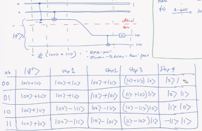
    • 1201+1211CNOTCNOT1201+CNOT1211\frac{1}{\sqrt{2}}|01\rangle + \frac{1}{\sqrt{2}}|11\rangle \xrightarrow{CNOT} CNOT\frac{1}{\sqrt{2}}|01\rangle + CNOT\frac{1}{\sqrt{2}}|11\rangle

Superdense-coding

  • Communicating between Alice and Bob

Partial Measurement

  • Assume you have ψ=1200i210+1211|\psi\rangle = \frac{1}{2}|00\rangle -\frac{i}{2}|10\rangle + \frac{1}{2}|11\rangle
    • First Qubit (count from left)
    • Split it into 0 and 1, and factorize:
    • =0(120)+1(i20+121)=|0\rangle\left(\frac{1}{2}|0\rangle\right)+|1\rangle\left(-\frac{i}{2}|0\rangle+\frac{1}{\sqrt{2}}|1\rangle\right)
    • =0ψ0+1ψ1=|0\rangle \otimes |\psi_0\rangle + |1\rangle \otimes |\psi_1\rangle
    • The probability that selected qubit is 0 is ψ022=(1/20)2=1/4|||\psi_0\rangle||_2^2 = (1/2|0\rangle)^2 = 1/4
    • The probability that selected qubit is 1 is ψ122=(i20+121)2=14+12=34|||\psi_1\rangle||_2^2 = \left(-\frac{i}{2}|0\rangle+\frac{1}{\sqrt{2}}|1\rangle\right)^2 = \frac{1}{4} + \frac{1}{2} = \frac{3}{4}
    • You can also rearrange the qubits (by rearranging all kets) to extract a particular qubit.

Deutsch's Algorithm

  • Uses functions f0,f1,f2,f3f_0, f_1, f_2, f_3 that inputs & outputs 1 bit

    • f is either constant / balanced (each output appears the same # of times; 0 half the time and 1 half the time)
    • f0f_0: Set to 0 (Constant fx)
    • f1f_1: Identity (Balanced fx)
    • f2f_2: Flip bit (Balanced fx)
    • f3f_3: Set to 1 (Constant fx)
  • pg25 Bf

  • Every BfB_f corresponds to a permutation matrix; second output outputs parity of b and f(a)

    • Bfab=abf(a)B_f|a\rangle |b\rangle = |a\rangle |b \oplus f(a)\rangle
    • if b=(01)|b\rangle = (|0\rangle - |1\rangle), then bf(a)=0f(x)1f(x)=(1)f(x)(01)|b \oplus f(a)\rangle = |0\oplus f(x) \rangle - |1\oplus f(x) \rangle = (-1)^{f(x)}(|0\rangle - |1\rangle)
    • if a=(01)|a\rangle = (|0\rangle - |1\rangle), then split f(x) by a's kets:
      • Bf((120+121)(120121))=Bf(120(01)+121(01))=B_f(\left(\frac{1}{\sqrt{2}}|0\rangle+\frac{1}{\sqrt{2}}|1\rangle\right)\left(\frac{1}{\sqrt{2}}|0\rangle-\frac{1}{\sqrt{2}}|1\rangle\right)) = B_f(\frac{1}{2}|0\rangle(|0\rangle-|1\rangle)+\frac{1}{2}|1\rangle(|0\rangle-|1\rangle)) =
      • 120(0f(0)1f(0))+121(0f(1)1f(1))=12(1)f(0)0(01)+12(1)f(1)1(01)=(12(1)f(0)0+12(1)f(1)1)(120121)\begin{aligned} \frac{1}{2}|0\rangle(|0 \oplus f(0)\rangle-&|1 \oplus f(0)\rangle)+\frac{1}{2}|1\rangle(|0 \oplus f(1)\rangle-|1 \oplus f(1)\rangle) \\ &=\frac{1}{2}(-1)^{f(0)}|0\rangle(|0\rangle-|1\rangle)+\frac{1}{2}(-1)^{f(1)}|1\rangle(|0\rangle-|1\rangle) \\ &=\left(\frac{1}{\sqrt{2}}(-1)^{f(0)}|0\rangle+\frac{1}{\sqrt{2}}(-1)^{f(1)}|1\rangle\right)\left(\frac{1}{\sqrt{2}}|0\rangle-\frac{1}{\sqrt{2}}|1\rangle\right) \end{aligned}
  • Permutation matrix: all entries are 0 or 1 and every row + column has exactly one 1 in it

    • A permutation matrix corresponds to a 1-1 function and is a unitary matrix
  • XOR / Parity identities: A =

    • B ⊕ ( A ⊕ B ) (commutative)
    • = B ⊕ ( B ⊕ A ) (associative)
    • = (B ⊕ B) ⊕ A (self-inverse)
    • = 0 ⊕ A (identity element)
    • \forall f(x) 0,1\in {0,1} 0f(x)1f(x)=(1)f(x)(01)|0\oplus f(x) \rangle - |1\oplus f(x) \rangle = (-1)^{f(x)}(|0\rangle - |1\rangle)
    • a,b0,1\forall a,b \in {0,1} (1)a(1)b=(1)ab(-1)^a(-1)^b = (-1)^{a\oplus b}
    • a0,1\forall a \in {0,1} H(12(0+(1)a1))=aH(\frac{1}{\sqrt{2}}(|0\rangle + (-1)^a|1\rangle)) = |a\rangle
    • Function in phase = "phase kick-back"
  • Simon's Problem

    • f(x) and f(y) follow the rule f(x)=f(y)<=>xy=sf(x) = f(y) <=> x\oplus y = s for some s0,1ns\in {0,1}^n (x and y are in same domain as s)
    • f(x) is 1-1 if s=0ns = 0^n
  • Modular Addition

    • lgN bit complexity because the addition of x and y will not exceed N length
  • Modular Inverse

    • Relatively prime / coprime: there is no integer greater than one that divides them both (that is, their greatest common divisor is one)
    • If you have a number x which is relatively prime to N, then it will have an inverse (it will have a y s.t. xy1(modN)xy \equiv 1 (mod N))
  • Definitions & Properties | - | Matrix Multiplication | h3 | |-|-|-| | Commutative | NO: AB \neq BA | data3 | | Associative | YES: (AB)C = A(BC) | data3 | | Distributive| YES: [A(B+C) = AB + AC] and [(B+C)A = BA + CA] | | Inversion | YES IFF SQUARE: AA1=A1A=InAA^{-1} = A^{-1}A = I_n